Cell culture
Human Jurkat cells Clone E6.1 (ATCC TIB-152) had been cultured in RPMI-1640 containing 10% fetal bovine serum (FBS) at 37 °C and 5% CO2. Culture medium became refreshed every 2–3 days and cells had been saved at densities between 0.5 × 10⁶ and a pair of × 106 cells per ml unless lysis or drug remedy.
Cell line authentication was performed using single nucleotide polymorphism profiling (Multiplexion).
Compound data
The information on the target sites of the 144 compounds included in this study was obtained from DrugBank Online (as of July 2023) and vendor specifications. Data regarding the clinical stage the compounds were in at the time the study was conducted were retrieved from ChEMBL (as of July 2023).
Compound remedy
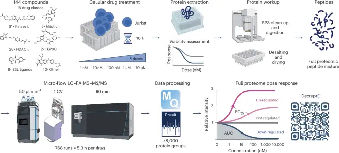
Compounds had been prediluted in DMSO and extra in culture medium interior a forty eight-deep-smartly plate. Per forty eight-deep-smartly plate, three DMSO controls had been added. For remedy, 4 × 10⁶ cells in RPMI-1640 medium supplemented with 10% FBS had been added on top of every compound predilution main to a remaining quantity of 2 ml and remaining remedy concentrations beginning from 10 µM to 1 nM in elephantine log10 steps, main to 5 doses for every drug (10 µM, 1 µM, 100 nM, 10 nM, 1 nM). Cells had been incubated for 18 h if no longer acknowledged otherwise at 240 rpm, 37 °C and 5% CO2. The next day, cells had been subjected to viability evaluation and lysis.
Confluency, viability and metabolic activity assessment
For determination of cell viability and metabolic activity after compound treatment, 100 µl of cell suspension per well was added to a 96-well plate containing 50 µl of IncuCyte Cytotox Dye (250 nM final concentration, Sartorius) and alamarBlue Cell Viability Reagent (10% final concentration (v/v), Invitrogen). The plate was placed into the IncuCyte live-cell imaging system (37 °C and 5% CO2) and cells were analyzed for cytotoxicity over a time course of 3 h (×10 magnification, scan mode was standard with 5 images per well, channel selection was phase contrast and fluorescence (300 ms acquisition time), scan interval was every hour). The integrated tool of IncuCyte (Standard Analyzer) was used for confluency and cytotoxicity analysis. After 3.5 h, metabolic activity was determined by fluorescence measurement of the AlamarBlue reagent using the fluorescence readout on the microplate reader FluoStar Omega (lex = 544 nm and lem = 584 nm, BMG Labtech).
For confluency and metabolic activity evaluation, the resulting values had been normalized to the mean values for the DMSO control. For cytotoxicity, the values had been corrected for differences in confluency, before normalizing the values to the mean values for the DMSO controls. Dose–response curves had been fitted to the data as described below (section ‘Curve fitting’).
Any small images displayed in the paper or in other locations had been exported from the IncuCyte system as shown and not further modified.
Cell lysis for protein extraction
To prepare cell lysate from untreated cells (for optimization purposes), cell suspension was centrifuged at 172g for 5 min at room temperature, washed with PBS (phosphate buffered saline, without calcium or magnesium) and pelleted before resuspension in lysis buffer (2% SDS, 40 mM Tris/HCl, pH 8, 95 °C).
Lysis of compound-treated cells became performed in 96-deep-smartly plates. Therefore, after 18 h of remedy time, forty eight-deep-smartly plates had been centrifuged (172g10 min, 4 °C), supernatant became discarded, cell pellets had been resuspended in PBS and transferred to a 96-deep-smartly plate. Cell pellets had been washed two more events with PBS and centrifuged to discard the supernatant sooner than lysis in 100 µl of lysis buffer.
For hydrolysis of DNA, lysate was heated to 95 °C for 10 min while shaking at 172g and trifluoroacetic acid was added to a final concentration of 1% (v/v) and incubated for 1 min while shaking. As a result, N-methylmorpholin (NMM) was added for neutralization to the hot lysate to a final concentration of 2% (v/v). Lysate was stored at −20 °C until further use.
Tissue and bacteria sample preparation
Mouse muscle (M. musculus) and Arabidopsis thaliana (A. thaliana) tissue samples were snap frozen in liquid nitrogen before homogenization using the TissueLyser II (Quiagen, 5 min, 30 Hz, using one stainless steel bead with a 5 mm diameter). Lysis buffer (4% SDS, 40 mM Tris/HCl, pH 8) was added after removing the bead and samples were sonicated using the Bioruptor Pico (Diagenode, 25 cycles with 30 s on/off). DNA hydrolysis was performed as described above using final concentrations of 2% trifluoroacetic acid and 4% N-methylmorpholin, respectively. Lysates were cleared by centrifugation (60 min, 4 °C, 21,000g). Supernatant lysate was stored at −20 °C until further use.
Escherichia coli (E. coli) and Pseudomonas aeruginosa (P. aeruginosa) had been grown in a shaker culture in Luria-Bertani medium at 37 °C, 300 rpm. When reaching an optical density of 0.5 and 0.6, respectively, cultures had been harvested by centrifugation (172g for 60 min, 4 °C) and washed twice with PBS. Lysis buffer was added to the pellet, followed by DNA hydrolysis as described above. Lysate was sonicated using the Bioruptor Pico (above) before clearance by centrifugation (60 min, 4 °C, 21,000g). Cleared lysate was stored at −20 °C until further use.
Isolation and sorting of T cells from healthy donors
Thrombocyte-depleted blood samples had been obtained from two healthy, voluntary human donors (male, age 26) after they gave written and informed consent. This study was approved by a vote from the ethics committee of the University Hospital München rechts der Isar (564/18S). Samples were transferred into 50 ml Falcon tubes, with each tube containing approximately 15 ml of blood. The Falcon tubes were then filled up to a total volume of 37.5 ml with PBS, and the blood was thoroughly mixed. To isolate peripheral blood mononuclear cells (PBMCs), a 12 ml layer of Pancoll was meticulously underlaid using a 24 ml syringe with an extended needle (G 20 × 2 3/4’; Ø 0.9 × 70 mm). As a result, the blood samples were subjected to centrifugation using a programmed gradient (acceleration of 7, deceleration of 1, 2, 7g for 20 min at room temperature). Following the gradient centrifugation, the plasma portion was discarded, and the PBMC-containing buffy coat was carefully collected. The PBMCs were then washed with 50 ml of PBS using centrifugation (441g for 5 min, at room temperature).
For cell separation, 107 PBMCs were resuspended in 40 µl MACS buffer (PBS, 1% FCS, 2 mM EDTA) and incubated with 10 µl antihuman CD4 beads for 15 min at 4 °C. As a result, PBMCs were washed with 15 ml of MACS buffer and centrifuged. CD4 T cells were positively enriched using the autoMACS Pro Separator. The flowthrough was retained and used for the isolation of CD8 T cells according to the CD4 T cell isolation protocol. Isolated T cells were cultured in RPMI-1640 containing 10% FBS and 1% penicillin and streptomycin (37 °C, 5% CO2) and were either subjected to HDACi treatment immediately or activated as described below.
HDACi treatment of peripheral T cells from healthy donors
For every population (CD4+/CD8+) a portion of cells was activated using Dynabeads Human T-Activator CD3/CD28 for T Cell Growth and Activation (Invitrogen) and incubated for forty-eight hours (37 °C, 5% CO2) before HDAC inhibitor (HDACi) treatment. Naïve T cells were subjected to treatment immediately after isolation and sorting. Regardless of activation status, cells were treated with various HDACi (5 doses for each drug: 10 µM, 1 µM, 100 nM, 10 nM and 1 nM) for 18 h, followed by viability, confluency and cytotoxicity evaluation as described above. Cell lysis, protein extraction followed by proteomic workflow and LC–FAIMS–MS/MS analysis was performed as described in the respective sections. For samples, where available material was limited, protein input was adjusted for tryptic digestion and obtained peptides were loaded on Evotips and analyzed on an Evosep-FAIMS-Exploris setup as described previously46 (for a complete list of instrument settings, see Supplementary Table 3).
Transcriptome sample preparation and diagnosis
For transcriptome diagnosis, Jurkat cells were treated according to the protocol described above. After 18 h, cells were lysed and total RNA was extracted using the ReliaPrep RNA Cell Miniprep Kit (Promega), according to the manufacturer’s protocol, and evaluated on a 2100 Bioanalyzer (Agilent Technologies). RNA library preparation was performed using the 3′ mRNA-Seq Library Prep Kit FWD with Unique Dual Indices (Lexogen) and was sent to Lexogen for gene expression profiling. Alignment of obtained reads was performed using the data processing pipeline provided by the manufacturer using the QuantSeq FWD pipeline and Homo sapiens (H. sapiens) genome annotation. The obtained alignments were trimmed, reads were counted and normalized. Dose–response curves were fitted to the data as described below (section ‘Curve fitting’).
SP3 sample preparation and tryptic digestion
Protein yield was determined by Thermo Pierce BCA (bicinchoninic acid) protein assays. All steps were performed according to the manufacturer’s protocol.
Before tryptic digest, detergent was removed by single-pot SP3 clean-up, following the protocol first described by Hughes et al.25 tailored to a Bravo Agilent liquid handling platform. In brief, lysate containing 200 µg of protein was mixed with 1 mg SP3 beads (50:50 mixture of Sera-Mag carboxylate-modified magnetic bead forms A and B (Cytiva Europe)) in a 96-deep-well plate and proteins were precipitated onto the beads in 70% ethanol in ddH2O (double distilled water).
The beads had been washed three times with 80% ethanol in ddH2O and once with 100% acetonitrile (ACN). Disulfide bonds had been reduced with 10 mM dithiothreitol for forty five min at 37 °C, followed by alkylation of cysteines with 55 mM CAA (2-chloroacetamide) for 30 min at room temperature in 100 µl of digestion buffer (2 mM CaCl2 in 40 mM Tris-HCl, pH 7.8). Trypsin (1:50 (wt/wt) enzyme-to-protein ratio) was added and proteins had been digested off the beads at 37 °C and 1,200 rpm overnight. For peptide recovery, the beads had been settled on magnets and the supernatant was transferred to a new 96-well plate. Beads had been washed by addition of 100 µl 2% formic acid in ddH2O and the supernatant was transferred to the collection plate. As a result, the samples had been desalted as described below.
Desalting and drying of peptides
Earlier than LC–MS/MS diagnosis samples had been desalted using hydrophilic-lipophilic balanced (10 mg of N-vinylpyrrolidon-divinylbenzol porous particles 30 μm, Macherey-Nagel) 96-smartly plates using centrifugation at 7g for 1 min unless specified otherwise. For this, hydrophilic-lipophilic balanced discipline fabric became primed with 500 µl of isopropanol, ACN and solvent B (0.1% formic acid in 70% ACN in ddH2O) and equilibrated with 1,000 µl of solvent A (0.1% formic acid in ddH2O) sooner than sample loading (by gravitation, 5 min). The sample flowthrough became reapplied to the plate and sure peptides had been washed with 1,000 µl of solvent A. Peptides had been eluted with 250 µl of solvent B (3 min, 7g; 1 min, 172g). Samples had been frozen at −80 °C, dried by vacuum centrifugation and saved at −20 °C unless LC–MS/MS dimension.
High pH reversed-phase fractionation
Here, 50 µg of peptides (A. thaliana for Extended Data Fig. 1i and Jurkat for Fig. 3b and Extended Data Fig. 4d–e) had been fractionated by frequent pH reversed-phase solid-phase extraction (reversed-phase sulfonate cartridge tips; 5 μl of polystyrene-divinylbenzene (PS-DVB) resin, Agilent) into six fractions using the Agilent AssayMAP Bravo pipetting system. The reversed-phase sulfonate cartridges had been primed, washed and equilibrated in accordance with the manufacturer’s protocol. Peptides had been reconstituted in 100 μl of 25 mM ammonium formate (pH 10) and loaded onto the cartridges. Peptides had been fractionated by increasing ACN concentrations (5, 10, 15, 20, 25, 30, 80%). The seven elution steps had been either combined into six fractions, combining the 5 and 80% fractions, or into four fractions. For four fractions, the 5 and 25%, the 10 and 30%, the 15 and 80%, and the 20% ACN fractions and the flowthrough had been combined. All fractions had been acidified with formic acid to a final concentration of 1%. Samples had been frozen at −80 °C, dried by vacuum centrifugation and stored at −20 °C unless LC–MS/MS analysis.
Microflow-LC–(FAIMS)–MS/MS measurements
All samples (with the exception of where indicated otherwise) had been analyzed on a microflow-LC–MS/MS draw using a Vanquish Neo extremely excessive-efficiency LC draw (Thermo Fisher Scientific) coupled to an Orbitrap Eclipse Tribrid mass spectrometer (Thermo Fisher Scientific) with or without installed FAIMS Pro Interface (Thermo Fisher Scientific). For a elephantine listing of ancient instrument tool, behold Supplementary Desk 3Materials.
Prior to analysis, samples were reconstituted in 0.1% formic acid, 2% ACN. For run optimization, the peptide concentration was determined using a Nanodrop instrument (Thermo Fisher Scientific) and the amount of peptide required for each run was injected accordingly. For drug profiling samples, half of the samples were injected per run (50 µg). For fractionated samples, all material was injected.
Chromatographic separation became performed by technique of notify injection on a 15 cm Acclaim PepMap 100 C18 column (2 µm, 1 mm inner diameter × 15 cm, Thermo Fisher Scientific) at a plug with the hump rate of 50 µl min−1. The column temperature became set apart to 55 °C. Solvent A became 0.1% formic acid in 3% DMSO in ddH2O, and solvent B became 0.1% formic acid and 3% DMSO in ACN. The gradients for diversified lengths can even be found in Supplementary Desk 3LC gradients.
Incorporation of FAIMS into microflow-LC–MS/MS
Because micro-LC separations generate noteworthy sharper peaks than nano-LC, the incorporation of FAIMS into microflow-LC–MS/MS draw critical to be evaluated from the bottom up. We first characterized the tool for peptide transmission at diversified compensation voltage (CV) values using a tryptic digest. With these data in hand, we next simulated how many and which CV values wants to be mixed for wonderful proteome protection. Simulations had been experimentally examined using LC gradient lengths between 15 and 180 min and we systematically when put next efficiency with and without FAIMS. For gradient events of 15, 30 and 60 min, simplest one CV atmosphere can even be meaningfully ancient attributable to CV switching takes sizable amounts of time. Regardless of LC events, FAIMS elevated the amount of identified protein groups at a given time or halved the MS time critical to carry out the identical depth of diagnosis when put next to the identical LC set apart-up but without using FAIMS.
Dimension without FAIMS installed
The OptaMax NG ion source (Thermo Fisher Scientific) with a heated electrospray ionization probe became ancient to spoil the information. The sprayer became positioned at middle spot in the x axis (left to handsome), at spot 1 in the y axis (front to abet) and between positions M and L in the z axis (probe peak).
The mass spectrometer was operated in data-dependent MS/MS, positive ion mode, using a spray voltage of 3.5 kV, a funnel radio-frequency lens value of 40, an ion transfer tube temperature of 325 °C and vaporizer temperature of 125 °C. The flow rates for sheath gas, auxiliary gas and sweep gas were set to 32, 5 and 0 l min−1 respectively.
A full-scan (MS1) was recorded from 360 to 1,300 m/z with a resolution of 120,000 in the Orbitrap in profile mode. The MS1 AGC target was custom set to 100% and the maxIT was set to 50 ms. Following the full scans, precursors were targeted for the MS/MS scans (MS2) if the isotope envelope was peptidic (monoisotopic precursor selection), the charge was between 2 and 6 and the intensity exceeded 1 × 10⁴. The MS2 quadrupole isolation window was set to 0.4 m/z. Peptide fragmentation occurred in the ion routing multipole by HCD with a fixed collision energy mode, the collision energy normalized to the precursor m/z and set with a collision energy of 28%. The MS2 scan was acquired in the Ion Trap with rapid scan rate in centroid mode and an defined first mass of 100 m/z. Additional MS2 properties as well as cycle events for different gradient lengths can be found in Supplementary Table 3MS settings.
Dimension with FAIMS installed
The identical ion source and probe as above were used, making use of the identical spray conditions. The mass spectrometer was operated in data-dependent MS/MS, positive ion mode, using a spray voltage of 4 kV, a funnel radio-frequency lens setting of 40, an ion transfer tube temperature of 325 °C and vaporizer temperature of 300 °C. The plug with the flow rates for sheath gas and auxiliary gas had been set to 40 and 5 l min−1 respectively. FAIMS was operated with standard temperature (inner and outer electrode 100 °C) and a static carrier gas flow with the flow of 3.5 l min−1. Dimension parameters were unchanged and the respective FAIMS CV was set to the critical value. For measurements of drug perturbed samples, the 60 min gradient was used with a series CV of −30 V.
If multiple internal CVs were used (for optimization), separate experiments were specified for the different CVs in the Tune method with the identical settings, except for the different CV value (the CV values used can both be read directly from the figures or the raw file names). This results in the MS looping through the specified experiments of the method, switching after every MS cycle (MS1 scan + MS2 scans). To ensure the data points and thus quantification quality were sufficient, the cycle time stated above was divided by the number of internal CVs used, leading to 0.75 s for 60 min (two CVs), 1.4 s for 120 and 180 min (two CVs) and 0.8 s for 120 and 180 min (three CVs).
Database hunting
The uncooked MS data information had been processed with MaxQuant v.1.6.2.10 (ref. 27) using the integrated Andromeda search engine and searched in opposition to the respective reference database (H. wise: downloaded from UniProt containing canonical and isoforms 24 August 2020; 75,776 entries, E. coli: downloaded from UniProt containing canonical and isoforms 1 July 2021; 4,713 entries, P. aeruginosa: downloaded from UniProt containing canonical and isoforms 1 July 2021; 5,563 entries, M. musculus: downloaded from UniProt containing canonical and isoforms 1 July 2021; 25,381 entries, A. thaliana: Araport11 genome unlock downloaded from Arabidopsis.org containing canonical and isoforms 16 June 2020; forty eight,359 entries).
Raw data from runs with multiple internal FAIMS CVs had to be split into separate files based on CV values before MaxQuant searches. These separate files were specified as different fractions, as for the normal reverse-phase fractions, of the same experiment in MaxQuant. Multiple injections of the same sample were specified as the same experiment. Standard MaxQuant search parameters were used. Trypsin/P was specified as protease, allowing up to a maximum of two missed cleavages. Carbamidomethylation of cysteine was specified as a fixed modification, whereas oxidation of methionine and protein N-terminal acetylation were considered as variable modifications. Where specified, mono- and di-methylation of arginine and lysine were enabled as variable modifications. The label-free quantification (LFQ) algorithm, with a default LFQ minimum ratio count setting of 1, as well as the iBAQ (intensity-based absolute quantification) algorithm, with log fit, were enabled where required. Where used, the Match-Between-Runs algorithm was enabled with default settings (0.7 min and 5 min for matching and retention time alignment window, respectively). The false discovery rate (FDR) was set to 1% at the protein and peptide spectral match level. For Prosit rescoring, the FDR was set to 100% at the protein and peptide spectral match level. The respective MaxQuant msms .txt and .raw files were rescored by Prosit. Peptides with q values ≤0.01 were retained and proteins were grouped based on the selected FDR method47. For MaxQuant output, proteins for which no unique peptide was found and thus were not distinguishable were aggregated into protein groups. For selected FDR protein group output, proteins are grouped at the gene level and only unique peptides are considered. For clarity, we refer to all such entities as proteins in the figures. Data analysis and visualization were performed using R (v.4.1.0) in RStudio (see Supplementary Table 3 for a complete list of all software used) and Microsoft Excel 365. Further refinement of plots was carried out in Adobe Illustrator CS6. Information on whether a dataset was rescored or not can be found on MassIVE (Data availability section).
Data processing and analysis
Curve becoming
For every protein–drug pair, the LFQ intensity relative to the median protein intensity in the DMSO controls was calculated for all drug concentrations. The same was done for every transcript–drug pair of the transcriptomic data using read counts. For the various viability metrics, the data were processed as described above. To these normalized data, a sigmoidal four-parameter log-logistic model (equation (1)) was fitted using the dose–response curve R package (v.3.0-1), where x is the log10 of the drug concentration, pEC50 is the negative log of the inflection point of the curve (denoted as the effective concentration 50; EC50), t is the top or low-dose plateau, b is the bottom or high-dose plateau, s is the curve slope between the plateaus and Y(x) is the observed protein ratio relative to the DMSO control at concentration x.
$$Yleft(xhandsome)=frac{t-b}{left(1+{10}^{left(sevents left(x-{mathrm{pEC}}_{50}handsome)handsome)}handsome)}+b$$
(1)
For each resulting model, descriptive parameters were extracted and reported. These included the optimized slope (s), top (t), bottom (b) and inflection point (EC50), as well as the area under the curve, the coefficient of determination (R2), mean absolute deviation, the predicted y value of the fitted curve at the highest concentration (end of curve, fold change) and the slope of a linear model fitted to the data.
Curve classification
To avoid manual annotation of more than 1 million dose–response curves, a random forest classifier was trained using the ranger R package (v.0.14.1). As a ground truth dataset, curves of two compounds had been manually annotated as up-, down- and nonregulated. The dataset was split into 80:20 for training and validation, respectively (training 11,562, validation 2,883, total 14,409). The input features were created from the values described above, along with the relative LFQ intensities and number of unique peptides for all concentrations and abundance percentile of the respective protein in the DMSO control. After hyperparameter tuning, the final model was trained with 1,200 trees, randomly selecting 15 independent variables at each split and splitting only nodes with a minimum size of 3. Variable importance mode was set to impurity and the Gini split rule was used. The model’s performance and quality were evaluated using the validation dataset, calculating precision, confusion matrices and ROC curves. The resulting classifier was used as a prefilter, plotting curves into separate PDFs and writing data into separate .txt files based on the predicted classes, thereby facilitating manual examination of all drug datasets. The same classifier was used for the dose–response curves of the drug perturbed transcriptome dataset. These regulated proteins were further analyzed to determine the mode of action of drugs.
Extra filtering
For further analysis, a protein was considered up- or down-regulated if it was classified as such and the fold change exceeded 1.5 for up-regulation and 0.7 for down-regulation. The same criteria were applied to all transcripts, retaining only observations where read counts were above 50 for all concentrations.
GO term enrichments
For the heatmap clustering of medication with identical effects, a GO term enrichment diagnosis became performed for every drug for my portion using the clusterProfiler R bundle (v.4.2.2.)forty eight. Every drug dataset became examined for enrichment of GO terms on all ranges (cell compartment, molecular feature and natural course of) both in up- and down-regulated proteins with the entire drug dataset because the background. P values had been corrected using the FDR ability and the q ticket in the discount of-off became set apart to 1. The enrichment outcomes for up- and down-regulation had been mixed, preserving the more critical entry for duplications. After combining the enrichment outcomes for all tablets, the q values had been log transformed, multiplied by −1 for GO terms enriched in down-regulation and z-scored for every GO term for my portion. The heatmap depicts the mixed, preprocessed GO term enrichment outcomes after hierarchically clustering of both rows and columns using Pearson correlation as a distance metric and Weighted Pair Crew Plot with arithmetic point out because the agglomerative formula. The GO term enrichment outcomes displayed in Extended Data Fig. 6a had been taken from the realm GO term enrichment diagnosis described above. For Extended Data Fig. 5d a brand new GO term enrichment diagnosis became executed (P ticket in the discount of-off, 0.05; P ticket correction, FDR ability; Subontology, Molecular Feature; total H. wise database as background).
Dose-dependent methylation
The search results for lysine and arginine methylation were challenging for dose–response curve fitting, similar to the process described for proteins and transcripts above. However, for each peptide–concentration–inhibitor combination, the intensity ratio of methylated to unmethylated form was calculated. The resulting value was then normalized to the respective DMSO control before proceeding as described above (section ‘Curve fitting’).
Simulation of target coverage relative to proteomic depth
For the simulation of target coverage across captured proteomic depth, we ranked all >8000 proteins in this study by their iBAQ values in all DMSO controls in descending order. To simulate varying proteomic depths, this list was truncated at the indicated ranks (number of identified proteins). For each drug, we then assessed how many of its targets were included in the resulting list and calculated the fraction of targeted proteins that were detected.
Replicate diagnosis
For the volcano plot displayed in Extended Data Fig. 2b assessing the quantitative reproducibility, the forty-eight DMSO controls had been randomly assigned into two equally sized groups. After median centering normalization of the LFQ intensities of the picked FDR gene neighborhood output and filtering for completeness in the dataset, a two-sided Student’s t-test was performed for all 4,694 proteins. P values had been corrected for multiple hypothesis testing using the FDR method using the R package fdrtool (v.1.2.17).
For the comparison of quantitative reproducibility between unregulated and regulated proteins using the 5 individual doses for every inhibitor as replicates, the LFQ intensities of the picked FDR gene neighborhood output had been normalized by median centering. The CoV was calculated across the 5 doses for every drug for every protein that was both classified as up- or down-regulated, or unregulated.
To evaluate the reproducibility of EC50 determinations, the curves for each protein for each drug replicate had been fitted as described above. For proteins being classified as up- or down-regulated in three out of four replicates per drug, the standard deviation of the pEC50s was calculated.
True-time RT–qPCR
For RT–qPCR diagnosis, cells were treated according to the protocol described above. After 18 h, cells were lysed, and total RNA was isolated using the Monarch Total RNA Miniprep Kit (New England Biolabs) according to the manufacturer’s instructions. RNA yield was determined using the Qubit fluorometer (Thermo Fisher Scientific). Complementary DNA (cDNA) was generated from 2 µg of RNA from each sample using the LunaScript RT SuperMix Kit (New England Biolabs) according to the manufacturer’s protocol. Additionally, no-reverse transcriptase controls were generated for each sample by omitting the reverse transcription step. After reverse transcription, the cDNA was diluted ~66-fold with nuclease-free ddH2O. qPCR was performed in triplicates on a CFX384 Touch Real-Time PCR Detection System (Bio-Rad Laboratories, Inc.) using 10 ng of cDNA per sample, the Luna Universal qPCR Master Mix (New England Biolabs) and the primer pairs as shown in Supplementary Table 3Primer listing. No-reverse transcriptase controls were measured in pools of all samples on each plate. Nuclease-free ddH2O was used as the no-template control for each assay. Cycling parameters were set to 95 °C (1 min), 40 cycles of 95 °C (15 s) and 60 °C (30 s with plate read on SYBR channel) each, and finally a melt curve was recorded from 60 to 95 °C with an increment of 0.5 °C per 5 s and SYBR channel plate reads after each increment. All samples treated with the same drug in addition to the DMSO control were measured on the same plate.
Analysis of RT–qPCR outcomes
Quantification cycle (Cq) and melting temperature (Tm) values were determined using the CFX Manager v.3.1 tool (Bio-Rad Laboratories, Inc.). The regression formula of the tool was used for Cq evaluation with baseline correction and curve fit enabled. The fold change in expression after treatment and the ratio of truncated to full-length transcript were calculated in Microsoft Excel 365 from the obtained Cq values for each sample using the 2-∆∆Cq formula49.
T cell activation assay
Activation status of HDACi-treated Jurkat cells was analyzed using TCR and/or CD3 effector cells (nuclear factor of activated T cells or NFAT) from a T Cell Activation Bioassay (Promega) with minor adaptations of the manufacturer’s protocol. Briefly, TCR/CD3 effector cells (NFAT) were incubated with HDACi (5 doses for each drug: 10 µM, 1 µM, 100 nM, 10 nM and 1 nM) for 16 h, followed by nonspecific activation via CD3 and/or CD28 using the Human Anti-CD3/CD28 T Cell Activation Kit (Cell Signaling Technology). After 5 h, receptor-mediated signaling was measured by luminescence using a microplate reader FluoStar Omega (BMG Labtech). Thus, the intensity of the luminescence signal corresponded to the intensity of receptor-mediated signaling. To assess the level of T cell activation, the luminescence signals were normalized to the DMSO control. Dose–response curves were fitted to the data as described in the section ‘Curve fitting’.
T cell aggregation diagnosis
The usage of the intense gentle photos of residing activated human T cells, bought using the IncuCyte live-cell diagnosis draw as described above, cell aggregates had been assigned and quantified (rely and situation in µm2). To this end photos had been processed by ilastik50a supervised machine studying image diagnosis tool bundle. The frequent aggregate dimension became calculated for every image by summing up the detected aggregate areas and dividing by the rely of aggregates per image, treating the 5 photos bought per smartly as replicates. To evaluate statistical significance of the HDACi prompted discount of moderate aggregate dimension, an diagnosis of variance take a look at became performed for every inhibitor for my portion, followed by a Tukey handsome critical differ ences put up hoc take a look at.
Reporting abstract
Additional information on research design is available in the Nature Portfolio Reporting Summary linked to this article.