Long-term intravital subcellular imaging with confocal scanning light-field microscopy

Intravital imaging^{1,2,3,4,5,6,7} is vital for studying diverse physiopathological processes, such as brain functions and immune responses, which necessitates high spatiotemporal resolution, high fidelity and low phototoxicity to capture fine structures and transient three-dimensional (3D) dynamics non-invasively^{8,9,10,11,12,13}. An essential difference between in vitro and in vivo imaging is the presence of intense background fluorescence originating from out-of-focus signals and autofluorescence in scattered tissue or densely labeled samples, which poses a fundamental constraint on the imaging fidelity^14,15,16. Confocal microscopy^17,18,19 is the most widely used technique to address this problem with optical sectioning. By rejecting the out-of-focus fluorescence with a pinhole, slit or pinhole array, only the in-focus photons within a very shallow depth of field (DOF) are captured, leading to high signal-to-background ratio (SBR) in intravital imaging. However, these confocal approaches inevitably reduce system parallelization indicated by the effective data throughput per unit of time and result in strong phototoxicity due to repeated excitation of out-of-focus layers and intense laser illumination during 3D imaging. In contrast, light-field microscopy (LFM)^{20,21,22,23,24,25,26,27,28,29} maximizes the parallelization with low phototoxicity by exciting and imaging the entire volume within an extended DOF. By incorporating line-confocal illumination, confocal light-field microscopy (cLFM)³⁰ not only can detect 3D photons in a parallel way but also suppress the background fluorescence out of the effective axial range. However, its Fourier LFM configuration fundamentally reduces the spatial resolution due to the loss of high-frequency information during pupil segmentation, restricting the application in observing subcellular dynamics. Recently, we proposed scanning LFM (sLFM)³¹ to increase the resolution up to the diffraction limit while maintaining the low phototoxicity by placing a drifting coded microlens array (MLA) at the image plane^31,32. Although sLFM enables high-speed multi-site aberration correction with digital adaptive optics to maintain subcellular resolution in multi-cellular organisms, it still faces severe degradation with the existence of strong background fluorescence.

To address this problem, we propose confocal scanning LFM (csLFM) to achieve aberration-corrected high-speed 3D subcellular imaging with both optical sectioning and low phototoxicity by developing a line-confocal scheme upon our sLFM³¹. With direct synchronization of an axially elongated line-confocal illumination and the camera rolling shutter of multiple rows, csLFM can selectively collect fluorescent signals from in-focus volume within a compact system. Compared to sLFM, csLFM achieves 15-fold improvement in SBR for high-fidelity imaging of densely labeled samples while maintaining the same effective axial coverage, near-diffraction-limit resolution in complicated environments and two orders-of-magnitude reduction in photobleaching over spinning-disk confocal microscopy (SDCM). We constructed both inverted and upright csLFM systems to demonstrate their applications in diverse species, including zebrafish, Drosophila and mouse. Although large-scale 3D neural recording is one of the key applications of LFM, our results show that the crosstalk from background fluorescence severely degrades the fidelity of calcium responses at the single-cell level, leading to reduced orientation selectivity to visual stimuli. csLFM effectively removes the crosstalk and achieves similar performance to two-photon microscopy but with lower excitation power even below 1 mW mm⁻² and much higher data throughput. Moreover, various subcellular dynamics are observed by csLFM in previously challenging environments, such as migrasome delivery in mouse spleen, retractosome generation in mouse liver and 3D voltage imaging at subcellular resolution in Drosophila with dense labeling, demonstrating its broad applications in the intravital study of large-scale intercellular interactions.

Principle of csLFM

To achieve both imaging parallelization and optical sectioning, we designed an elongated line-confocal illumination^33,34,35 based on sLFM³¹. The camera rolling shutter is synchronized with the scanning illumination at high speed as the confocal slit to filter out background fluorescence without sacrificing the imaging speed in a compact system (Fig. 1a and Supplementary Fig. 1). To facilitate confocality, we set the slit size the same as the height of rolling shutter. The accurate synchronization contributes to a moving mask on light-field images followed by an integration process during exposure, which modulates the point spread functions (PSFs) at camera frame rate (Fig. 1bSupplementary Fig. 2 and Methods). The MLA is placed at the imaging plane for light-field detection, along with a piezoelectric tip and tilt platform for high-speed periodic drifting to address the tradeoff between spatial resolution and angular resolution in LFM³¹ (Supplementary Video 1). After data acquisition, iterative tomography with digital adaptive optics³¹ same as previous sLFM can be applied for aberration-corrected 3D reconstruction with the modified confocal PSF. By keeping the photons focused within an extended DOF, csLFM provides an efficient way for 3D sensing with elongated PSFs along different angles (Fig. 1c). Therefore, the design of silt size entails a holistic assessment of the photon efficiency, axial coverage and background rejection performance. Only photons falling beyond the effective volume range need to be eliminated, which is different from traditional confocal microscopy requiring a small pinhole size for a shallow DOF. When we reduce the slit size together with the height of rolling shutter, csLFM will first maintain the same DOF and then gradually lose its effective axial coverage (Supplementary Fig. 3a–g). If we do not consider confocal illumination in PSF modeling, there will be artifacts at the out-of-focus planes during 3D reconstruction, especially for small slit sizes (Supplementary Fig. 3h, i). On the contrary, increasing the slit size will loosen the confocal constraint, degrading the capability of background rejection as indicated by the numerical simulations (Supplementary Fig. 4a–g). Similar optical sectioning can be obtained when the slit size is smaller than 11-times Airy units (AU) of the whole-objective numerical aperture (NA). Consequently, to maximize the 3D photon efficiency for low phototoxicity while maintaining the high SBR, we set the slit size as 11 AU for the angular resolution of 13 × 13 in csLFM, corresponding to the 13 × 13 sensor pixels after each microlens (Supplementary Fig. 4h, i). The axial coverage remains almost unchanged relative to sLFM with an effective DOF of 15 μm for 1.4-NA objective and similar optical sectioning capability compared to the silt size of 1 AU (Supplementary Figs. 3c–f and 4g).

By changing different background levels in numerical simulation, csLFM quantitatively achieved 12-dB improvement in SBR over sLFM (Supplementary Fig. 5). Although our previous study of computational background suppression³⁶ can alleviate background contamination to some extent, the background fluorescence cannot be eliminated and will further reduce the axial resolution with the existence of strong background fluorescence (Supplementary Fig. 6). More importantly, the shot noise is positively correlated with the measured intensity, so it is difficult to be removed computationally. By physically rejecting the background fluorescence, csLFM can effectively increase the signal-to-noise ratio (SNR) to distinguish minute structures with subcellular resolution (Fig. 1 d and Supplementary Fig. 7). One of the key advantages of sLFM is multi-site aberration correction with digital adaptive optics. Spatially non-uniform aberrations can be estimated based on the local disparities between different angular components and then corrected during 3D reconstruction with an accurate PSF model. However, strong background fluorescence will deteriorate the accuracy of wavefront estimation, leading to severe artifacts and reduced resolution (Supplementary Fig. 8). csLFM can address this problem because it effectively extracts signals from the background. Another challenge arises from the highly dynamic samples, leading to motion artifacts during physical scanning. Both time-weighted algorithm³¹ or optical-flow-based correction³² are also applicable to csLFM to eliminate the motion artifacts while maintaining high spatial resolution (Supplementary Fig. 9).

Experimental characterization and analysis

For experimental validations, we compared csLFM with sLFM³¹ and cLFM³⁰ on the same system (Methods) and state-of-the-art intravital microscopy, such as SDCM and two-photon microscopy. We implemented cLFM³⁰ here with line-confocal illumination without two-dimensional (2D) periodic scanning. First, we evaluated the background rejection capability by imaging 500-nm-diameter fluorescence beads randomly distributed in a 3D tissue-mimicking phantom made of intralipid and agarose by different methods (Fig. 2a). Background fluorescence g radually overwhelmed the intensity of in-focus beads as the penetration depth increases, which degraded the imaging performance and limited the depth of sLFM (Supplementary Fig. 10a–c). Under different concentrations of intralipid, csLFM obtained an overall 12-dB improvement in terms of SBR with deeper penetration depth and about three-fold narrower lateral full width at half maximum (FWHM) profile along beads in raw measurements than sLFM (Fig. 2b). When compared to traditional slit confocal microscopy, csLFM captures four-dimensional (4D) spatial-angular measurements with an extended DOF along multiple angular PSFs. Therefore, the background fluorescence in the other orthogonal direction can still be distinguished based on the disparities between different angular views, achieving computational rejection of background fluorescence³⁶. The statistical plots indicate that csLFM can achieve similar performance to SDCM (Andor Dragonfly 200) in terms of SBR (Fig. 2c and Supplementary Fig. 10d). Similar results can be obtained when we used an upright system to image vascular structures in the brain of an awake wild-type mouse injected with AF647 dye. By increasing the SBR, csLFM increased penetration depth from 140 μm to 280 μm in mouse cortex with more uniform resolution performance than sLFM (Supplementary Fig. 11).

Next, we imaged endogenous immune cells in a mouse spleen (Fig. 2d). On the one hand, there were many dense cells distributed at multiple layers of the spleen parenchyma with strong autofluorescence, causing background contamination in sLFM. On the other hand, cLFM achieved higher contrast but with low resolution. csLFM addressed both problems and distinguished subcellular structures, such as retraction fibers, with substantial SBR improvement (Fig. 2d, e). Then, we imaged a 300-μm-thick Thy1-YFP mouse brain slice (Supplementary Fig. 12a,b and part III of Supplementary Video 1). Even with dense dendrites and synapses intricately interlacing in 3D space, csLFM could distinctly resolve fine structures swamped in sLFM (Supplementary Fig. 12c,d). Because the background fluorescence is highly non-uniform, it is difficult to be removed by simple background subtraction (Supplementary Fig. 13). We further imaged the same thick brain slice to compare the imaging performance among csLFM, SDCM and two-photon microscopy. The objective NA was selected closely. Due to the resolution limit, two-photon microscopy exhibited about 1.8 times lower resolution than csLFM, and the axial resolution is over two times worse, making it unable to clearly distinguish minute structures. In contrast, csLFM can achieve nearly the same performance as SDCM. csLFM also obtained the imaging speed improvement of about 20 times than SDCM and two-photon microscopy, showing its higher data throughput through 3D parallel detection (Supplementary Fig. 14). In addition, we quantitatively characterized the resolution of csLFM by imaging 100-nm-diameter fluorescence beads. Our results show that csLFM reaches near-diffraction-limit resolution both laterally and axially within a 10-μm axial coverage (Fig. 2f and Supplementary Fig. 15). Compared to unscanned cLFM, csLFM enhanced the lateral resolution by over three times and the axial resolution by over two times. Such a high resolution is further verified by calculating the coefficients of Fourier ring correlation (FRC) based on the intravital images with about 295-nm lateral resolution for csLFM, which is even better than sLFM with the existence of strong background (Fig. 2d).

Although csLFM uses the rolling shutter to block out the out-of-focus photons, it still maintains high data parallelization within the effective DOF due to the elongated line-confocal illumination. By imaging the same fixed cell within the DOF under the same excitation power and frame dwell time, csLFM can capture similar numbers of photons compared to sLFM with a high photon efficiency of approximately 85% (Supplementary Fig. 16). In this case, csLFM can maintain the low-phototoxicity advantage of sLFM. On the contrary, the entire volume is excited in SDCM, but only the photons from a 2D layer with a small DOF can be collected by SDCM due to the presence of a pinhole or pinhole array to reject the out-of-focus photons (Fig. 2g). In contrast, the emitted photons from an extended DOF are effective in csLFM. If under the same excitation intensity, much more effective photons are collected by csLFM and sLFM than SDCM. To obtain similar photon outcome, more exposure time is required for SDCM compared to csLFM. For verification, we imaged immune cells labeled by flow antibodies in a living mouse spleen, which would be bleached quickly under intense excitation light in SDCM. Therefore, when imaging continuously at the same rate and average power intensity with similar photon counts for both methods (more exposure time required for SDCM; Supplementary Table 1), quick photobleaching appeared in the kymographs (y–t projections) of SDCM results, whereas csLFM exhibited no apparent bleaching for over 5 h (Fig. 2h,i). Even if the laser intensity was intentionally increased by a factor of 5, csLFM showed only slight photobleaching with the decay time 100-fold longer than that of SDCM (Fig. 2j).

Collectively, csLFM achieves high-fidelity high-speed 3D imaging with optical sectioning in complicated environments while maintaining subcellular resolution and low phototoxicity.

Intercellular immune behaviors in living mouse spleens

Intravital imaging is critical to understand how the immune system works collaboratively in native states. A multitude of immune cells actively migrate and interact with each other. During the migration and interaction, immune cells leave long and thin retraction fibers and migrasomes to facilitate intercellular communication. These orchestrate dynamic and complicated cooperative behaviors to regulate immune responses^8,37. The mammalian spleen is recognized as a prominent organ of the immune system, housing abundant resident or transient immune cells involved in executing immune reactions. However, the spleen remains a challenging environment for subcellular imaging due to its dense tissue, strong background fluorescence and sensitivity to photodamage^38,39. csLFM exactly fills this niche.

We then compared csLFM to sLFM and cLFM by imaging immune cells in living mouse spleens. First, F4/80 and NK1.1 antibodies were intravenously injected into an anesthetized mouse to label macrophages and natural killer (NK) cells. Macrophages have a large size of over 20 µm and are broadly distributed in multiple compartments of the spleen⁴⁰leading to strong background during wide-field excitation (Fig. 3a). Although cLFM suppressed the background, the resolution would inevitably be reduced (Fig. 3b). On the contrary, csLFM resolved subcellular structures with considerable SBR improvement, which could be used to investigate migrasome functionality⁴¹ (Fig. 3c and part I of Supplementary Video 2). The delivery of migrasome in mammals was reported previously^31,42but it is confined to one type of immune cell (neutrophil). Whether migrasome could be a messenger between multiple immune cells is unknown. In this experiment, csLFM revealed that NK cells actively migrated in mouse spleen and sometimes interacted with macrophages through cellular protrusion extensions. When adhering to macrophages, NK cells generated retraction fibers and produced migrasomes inside the macrophages (Fig. 3d–g and part II of Supplementary Video 2). Similar cell-contacting processes through migrasomes were also validated by using a recently developed two-photon microscopy with a theoretical resolution of approximately 500 nm (ref. ⁴²) but at a smaller data throughput fundamentally limited by the fluorescence decay time (Supplementary Fig. 17). Although the functions of immune-cell-derived migrasomes are still to be determined, we speculate that the delivery of migrasomes may be a collaborative mechanism of signaling, which probably strengthens the immune surveillance system.

Next, we further explored the intercellular communications between dendritic cells and T cells. With the low phototoxicity, csLFM sustainably monitored the spleen microenvironment over 4 h at high speed. Reduced background clearly unveiled cell shapes, whereby 158 highly motile immune cells could be continuously tracked (Fig. 3h). More interestingly, we found that a dendritic cell and a T cell were entangled and interacted. They showed very frequent contacts through elongating retraction fibers, as if talking and dancing with each other (Fig. 3i and Supplementary Video 3). Such discoveries reveal that different types of immune cells may communicate and work collaboratively through retraction fibers to enhance the innate adaptive immune systems. The retraction fibers produced by frequent interactions of dendritic cells and T cells were counted, suggesting that cell-to-cell contacts via fibers might be a common occurrence in the mammalian immune system with, on average, a single fiber per cell pair (Fig. 3d–l). The successful application of csLFM to spleen imaging provides an insightful way to better understand complex subcellular interactions and collaborative behaviors of endogenous immune cells and organelles and also demonstrates its potential in observing other mammalian organs.

Retractosome biogenesis in mammals

With the high spatiotemporal resolution, our previously developed sLFM has made great progress in liver imaging, where the formation, division and delivery of migrasomes have been fully studied³¹. Different from migrasomes, retractosomes are newly discovered extracellular vesicles that have smaller sizes, ranging from 50 nm to 250 nm, compared to migrasomes, which is too small for two-photon imaging to resolve clearly, and may play important physiological roles⁴³. Although the existence of retractosome structures has been validated in vitro by SDCM with a few images, the function diversity needs to be explored in mammals with timelapse videos. Low phototoxicity, high resolution and high SBR are also required, because retractosomes are small and very susceptible to light. However, in the low-light condition, Poisson-dominated noises originating from the background intensity would overwhelm minute structures, such as retractosomes, and cause artifacts in sLFM (Fig. 4a,b).

To address this problem, we applied csLFM to image the mouse liver with both neutrophil marker (Ly6G) and vessel marker (wheat germ agglutinin (WGA)) under low excitation light for continuous imaging (Supplementary Table 1). By removing the background with better contrast, csLFM enabled a clearer visualization of vascular structures and subcellular dynamics than sLFM and cLFM (Fig. 4a,b and Supplementary Video 4). We then observed that a neutrophil migrated fast along the vessel, and numerous retractosomes were generated from broken-off retraction fibers (Fig. 4c). The intensity profile across a retractosome was plotted to demonstrate the near 300-nm resolution of csLFM in vivo. In another living mouse liver, a similar phenomenon was also observed, in which large quantities of retractosomes were produced and left behind in vessels after the retraction fiber was pulled out at the trailing edge of a neutrophil (Fig. 4d). These retractosomes were distributed as a string of beads, all detected with sub-micron diameters by csLFM, whereas cLFM misidentified them as larger structures spanning several microns (Fig. 4e). It should be noted that the measured diameters by csLFM might be slightly larger than the actual values because the retractosome size is close to the diffraction limit. Nevertheless, csLFM could still accurately preserve the morphology of delicate retractosome structures and distinguish them from the migrasome, which was usually 0.5–2 μm in diameter. Retractosomes were found more in number and smaller in size than migrasomes in mammals. We anticipate that, in the future, csLFM will be further used to investigate how retractosomes or other small vesicles are involved in immune responses.

High-fidelity high-speed 3D neural recording with reduced crosstalk in vivo

One of the typical applications of LFM is high-speed 3D neural recording. However, tissue scattering and dense fluorescence labeling introduce strong crosstalk contaminations during parallel detection, leading to a fundamental tradeoff between the number of neurons recorded simultaneously and the data fidelity. By increasing the spatial resolution and rejecting the background fluorescence, csLFM reduces the crosstalk while maintaining high 3D imaging speed (Fig. 5a).

To verify the advantages, we constructed an upright csLFM system equipped with a ×25/1.05-NA water immersion objective (Supplementary Fig. 18 and Methods) and observed calcium activities at the cortical layer 2/3 in an awake mouse expressing genetically encoded GCaMP6f (Ai148D). To increase the DOF, the slit size was set as 26 AU for higher angular resolution of 21 × 21 in the upright system⁴⁴. We compared the performance of sLFM and csLFM by imaging the identical region of interest (ROI) at 20 volumes per second (VPS; Supplementary Video 5). The cLFM counterparts were extracted from raw data of csLFM and analyzed. We used the CNMF algorithm⁴⁵ to extract the calcium traces at single-cell level. Given the relatively large size (~10 μm) of neurons and sparse distribution in mice, the functional traces extracted from cLFM results resembled those obtained with csLFM, yet distinguishing subcellular dendritic structures was difficult for cLFM (Supplementary Fig. 19a). Compared to sLFM, though, csLFM exhibited much more identified spike numbers and higher ΔF/F₀ amplitudes with better contrast (Fig. 5b,c). Applying background subtraction to sLFM data moderately improved the spike amplitude; however, it could not identify the sufficient number of neurons and spikes as in csLFM (Supplementary Fig. 19b,c). Some spikes engulfed by the background are difficult to recover.

To further analyze the data fidelity for neuroscience applications, we recorded the calcium dynamics in primary visual cortex under multiple rounds of visual stimuli with a moving grating (Fig. 5d). It is a classical experiment to measure the tuning properties of neurons responding to visual stimulus, which has been widely verified by electrophysiology and two-photon imaging^46,47. Except for better contrast in csLFM, we found that the same neurons with a sharp tuning curve in csLFM showed broadened curves in sLFM due to strong background crosstalk (Fig. 5e,f). In addition, many weak responses are flooded in the increased baseline signal in sLFM, which has been well retrieved in csLFM. The inter-class distances of csLFM were larger than those of sLFM during clustering (Fig. 5g,h). We further calculated the orientation selectivity index (OSI) for the neurons (Fig. 5i). Across four mice independently observed by sLFM, only 25% of all visually responsive neurons had orientation tunings larger than 0.8, whereas approximately 52% had OSIs larger than 0.8 in csLFM data on the same mice. The latter OSI distribution was similar to the results obtained by 2D imaging with a two-photon microscope (Fig. 5j and Supplementary Fig. 20), which also accords well with previous studies⁴⁸.

Because csLFM does not rely on any sample prior, it can be generally applied to diverse species with different indicators. Next, we recorded timelapse calcium transient of the whole brain in a zebrafish larva expressing genetically encoded GCaMP6s (here: GCaMP6s). The zebrafish brain contains a high density of neuron populations in foreground and background layers with small neuronal size, requiring high resolution to identify single cells clearly. After improving spatial resolution and rejecting out-of-focus light, more neurons were identified with better resolution and higher fidelity in csLFM than in cLFM and sLFM (Fig. 6a–d and Supplementary Video 6). Similarly, we imaged a craniotomized Drosophila expressing genetically encoded GCaMP7f (nsyb-Gal4×UAS-jGCaMP7f) in vivo at 60 VPS. The Drosophila brain is very different from mammalian and zebrafish brains in morphology, and its dense labeling leads to an intense background and low resolution, which is ameliorated by csLFM (Fig. 6e). We gave the Drosophila multiple rounds of odor stimuli, to motivate the calcium responses. Approximately two-fold increase in spike amplitude was observed, thereby verifying the effectiveness of csLFM (Fig. 6f,g).

Voltage indicators present more direct measurements of neural activities at higher speed but also pose more challenges for microscopy⁴⁹. Usually, very sparse labeling is used to increase the contrast for the recording of single-trial action potentials in vivo⁵⁰. Here, we performed volumetric voltage imaging in an awake behaving Drosophila (TH-Gal4×UAS-pAce) at a depth of 100 μm and speed of 150 VPS by labeling almost all dopaminergic neurons densely. Due to the ultrafast voltage transients, the image plane drifting was replaced by the virtual scanning network (Vs-Net) that we proposed previously⁵⁰ to achieve a higher temporal resolution. Compared to sLFM, csLFM reduced the background and improved the image contrast (Fig. 6h and Supplementary Video 7). Notably, some spontaneous voltage potentials drowned by the background in sLFM can be recognized by csLFM with high fidelity (Fig. 6i). csLFM obtained nearly a three-fold increase in identified spike number and 1.5 times enhancement in spike amplitude quantitatively (Fig. 6j,k). With its commendable performance and versatility, csLFM shows tremendous potential as a tool for large-scale neural recording at high fidelity.

In the present study, we combined concepts from line-confocal imaging and sLFM to address the inherent tradeoff between data parallelization and fidelity originating from background fluorescence. Through comprehensive integration spanning wave optics, synchronization of scanning light-sheet illumination and a camera rolling shutter and 3D reconstruction algorithm, csLFM offers a compact solution to retrieve effective signals from severe background and shot noises, and it achieves intravital 3D imaging in mammals with subcellular resolution and low phototoxicity at high fidelity up to camera frame rate.

csLFM stands out as a distinctive technology in comparison to other advanced microscopes. Light-sheet microscopy could effectively eliminate background light with minimal photobleaching by exciting only the in-focus 2D plane, ensuring high-sensitivity recordings during prolonged imaging of transparent samples, such as embryo and cleared tissue^13,51,52. With very thin illumination sheet such as lattice light-sheet microscopy, light-sheet microscopy can have better axial resolution than csLFM, which is still limited by the missing cone problem. However, light-sheet microscopy faces several constraints in mammalian imaging, such as the tradeoff between sheet thickness and length for wide field of view (FOV) imaging, susceptibility to tissue scattering and more axial scanning required for 3D imaging due to the small DOF as compared to csLFM. Two-photon imaging has an intrinsic advantage in deep tissue observation due to nonlinear excitation with longer wavelength, with broad applications for deep layer neural recording⁵³ and innate immune responses³⁷. However, the diffraction limit of two-photon microscopy is approximately 500 nm, making it challenging for monitoring behaviors of small organelles, such as the formation processes of retractosomes. Furthermore, similar to confocal microscopy, two-photon microscopy requires sequential scanning of a focal spot, collecting only in-focus photons with unnecessary heat damage to out-of-focus planes. The data throughput of two-photon microscopy is fundamentally limited by the fluorescence decay time and laser repetition rate, which is much smaller than the csLFM with imaging sensors of a large pixel number. In addition, two-photon microscopy usually requires a femtosecond laser, which is more expensive than the compact low-cost system of csLFM. Although csLFM cannot maintain high resolution in deep tissue, such as a depth of approximately 300 μm in mouse cortex, its high-speed, high-resolution, high-fidelity and low-phototoxicity features confer advantages in observing the large-scale behaviors of organelles in mammals and high-throughput recording of functional responses and intercellular interactions.

Several extensions are anticipated to csLFM. First, the snapshot DOF of csLFM can be further enhanced with wavefront coding or multi-focus excitation⁵⁴ up to the working distance of the objective lens. By customizing better objective lenses, the working distance can be further increased—for example, 20 mm for a 0.5-NA objective⁵⁵. Axial scanning³⁶ could also be used to increase the axial coverage of current csLFM at the cost of temporal resolution (Supplementary Fig. 21). Second, more accurate modeling of the scattering process in csLFM would be beneficial to increase the penetration depth and enable more quantitative imaging in deep tissue. Longer-wa velength imaging⁵⁶ or multi-photon light-field detection by manipulating the excitation light beam⁴² can also reduce the scattering effect. Third, implanting denoise algorithms^57,58 into csLFM can further reduce the excitation power, fulfilling the long-term observation of organisms very sensitive to light doses. Fourth, the imaging speed of csLFM is limited mainly by the camera frame rate, which can be increased with smaller ROI or faster cameras. Fifth, as a computational imaging method, csLFM requires more time for iterative reconstruction, which is expected to be further accelerated by deep learning methods⁵⁹.

Experimental setup

The inverted system

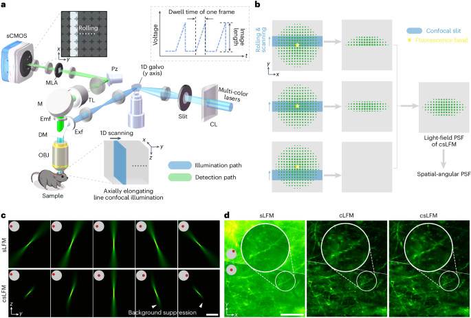
We made hardware modifications based on the inverted sLFM system reported in our previous work³¹. Our system serves as an add-on to a commercially available inverted microscope (Zeiss, Observer Z1), with the configuration of a ×63/1.4-NA oil immersion objective (Zeiss Plan-Apochromat ×63/1.4 Oil M27). In this way, our csLFM system can be compatible with standard sample holders for wide-field microscopes without any modifications. A scientific complementary metal-oxide-semiconductor (sCMOS) camera (Andor Zyla 4.2 PLUS), which has both global shutter mode and rolling shutter mode, was employed to collect fluorescent signals, with the pixel resolution of 2,048 × 2,048 and the pixel size of 6.5 μm. In global shutter mode, all pixels are simultaneously active during the exposure time. While in rolling shutter mode, a pixel window consisting of only a few adjacent pixel lines is actively exposed at one time and serially moves across the entire image sensor. In the detection path, we inserted a commercial MLA (RPC Photonics MLA-S100-f21) with a pitch size of 100 μm and a focal length of 2,100 μm at the image plane, which were then relayed by a pair of lenses with magnification of 0.845. In this way, each microlens covers exactly 13 × 13 camera pixels, achieving the angular resolution of 13 × 13. A piezoelectric tip and tilt platform (PI S-340 Piezo Tip/Tilt Platform) was used to drift the image plane periodically before the emission light enters the MLA. For cLFM acquisition, the platform was kept unscanned. In the illumination path, the beam output from multi-channel lasers (Coherent, OBIS 405/488/561/640) was first collimated by a convex lens and then modulated by a cylindrical lens (Thorlabs, LJ1363L2-A) into a thin light sheet along the x–z plane of the sample. The cylindrical lens played a role in improving laser efficiency. Next, the light-sheet beam passed through an optical slit with the specific width of 325 μm (~11 AU at the conjugate image plane), which sat approximately 100 mm in front of the back focal plane of the cylindrical lens, to generate an axially elongated line-confocal illumination. The offset distance makes the beam almost uniform within a 15-μm axial range in the object space, so the optical slit can act as a beam-shaping device to provide confocality (Supplementary Fig. 2a,b). A pair of relay lens and a y axis galvo (Thorlabs, GVS211) were implemented to scan the illumination beam and transmit it from the slit to the conjugated object plane. The multi-color fluorescence imaging was carried out with a multi-channel filter module, including a dichroic mirror (Chroma ZT405/488/561/640rpcv2) and filters (Chroma ZET405/488/561/640xv2 and Chroma ZET405/488/561/640mv2). When acquiring confocal scanning light-field images, the camera, galvanometer, piezoelectric platform and lasers were synchronically triggered using a controlling box (National Instruments, USB-6363) and our customized LabVIEW (2019 version) programs (Supplementary Fig. 1). During the acquisition of one image, a galvo translates the illumination beam, synchronized with the exposure of rolling shutter, beginning at the topmost pixel row and moving across the entire sensor region until the last row. Specifically, we drove the one-dimensional (1D) illumination galvo by a saw-tooth voltage signal and controlled the camera, lasers and piezoelectric platform using step-function voltage signals synchronically. Note that the triggered voltage should be precisely calibrated, so that the center of axially elongated line-confocal illumination is always coincident with the center of rolling window during the acquisition. The maximum beam deflection should exactly correspond to the first and last rows of the camera and the intermediate beam position moved linearly with the angle scanning of galvo. The data shown in Figs. 1–4Supplementary Figs. 2–8, 10, 12, 13, 15, 16 and 21 and Supplementary Videos 2–4 of this paper were captured by the inverted system.

The upright system

We additionally built an upright system for intravital imaging of animals’ brains. We constructed a customized microscope using Thorlabs Cerna series, with a ×25/1.05-NA water immersion objective (Olympus, XLPLN25XWMP2) and an infinity-corrected tube lens (Thorlabs, TTL180-A) to cover a larger field of view. A sCMOS camera (Teledyne Photometrics Kinetix) with larger photosensitive area, faster speed and higher quantum efficiency was used. The camera pixel size is also 6.5 μm. To achieve imaging in deeper tissues, we customized an MLA with the larger pitch size of 136.5 μm and focal length of 2,800 μm, which exactly covers 21 × 21 pixels with the 1:1 relay lens between the MLA and the camera. The more angles we capture, the larger effective DOF can be achieved, and it is more suitable for deep imaging in mammalian brains. Accordingly, we customized another optical slit with larger width of 650 μm (~26 AU at the conjugate image plane) to increase axial coverage. Another relay lens with magnification of 1.64 was attached between the tube lens and the MLA to match NA between the objective and the MLA⁴⁴. The piezoelectric tip and tilt platform in the upright system was replaced with a more affordable one (Core Morrow P33.T2S) that still met precision needs. For cLFM acquisition, the platform was kept unscanned. Other components of the upright system, including lasers, filter modules, cylindrical lens, 1D illumination galvo and the synchronous control procedures, are consistent with the inverted system. The data shown in Figs. 5 and 6Supplementary Figs. 9, 14, 19 and 20 and Supplementary Videos 5–7 of this paper were captured by the upright system.

Detailed imaging conditions and parameters for all fluorescence experiments, including the fluorescence label, laser, excitation power, line exposure time, total dwell time, imaging speed, system mode, angular resolution, objective and confocality parameters, are illustrated in Supplementary Table 1.

PSF derivation for csLFM and principle of background suppression

In sLFM³¹the spatial-angular measurements of an arbitrary 3D point from object space with lateral coordinates of p = (p_x, p_y) and axial coordinate of p_z can be represented as

where x₀ = (x₀, y₀) denotes the center position of the microlens and x = (x, y) and u = (u, v) denote the relative lateral displacement to the center position at the native image plane and the sensor plane, respectively. ({U}_{{p}_{z}}({bf{x}}-{bf{p}})) denotes the complex field at the native image plane derived by the Debye theory; n is the refractive index; l is the wavelength of emission light; d_l and f_μlens are the pitch size and focal length of MLA; d_s is sensor pixel size; rect(·) is the 2D rectangle function; and F(·) is the 2D Fourier transform. Here, we temporarily ignore discrete property of detector pixels and obtain the expression of ({W}_{{p}_{z}}) in the continuous domain, which can be represented as

Note that u is limited by the microlens pitch, and x₀ is a discrete variable with a period of microlens diameter. So, x₀ + u can represent every point at the sensor plane, which is named sensor coordinates—that is, (tilde{{bf{x}}}=(tilde{x},tilde{y})={{bf{x}}}_{{bf{0}}}+{bf{u}}). (h{s}_{{p}_{z}}({bf{p}},{{bf{x}}}_{{bf{0}}},{bf{u}})) can be represented as (h{s}_{{p}_{z}}({bf{p}},{{bf{x}}}_{{bf{0}}}+{bf{u}})) (=h{s}_{{p}_{z}}({bf{p}},tilde{{bf{x}}})).

The optical slit is not exactly at the back focal plane of the cylindrical lens in csLFM setup. We thereby assume that the beam passing through the slit has a uniform pattern with a finite size. As shown in Supplementary Fig. 2bthe axially elongated line-confocal illumination can be approximated as a collimated sheet and represented by a rectangle function at each p_z plane. The illumination is scanned along the p_y axis while rolling shutter is sliding on the (tilde{y}) axis (Supplementary Fig. 2c). When the width of illumination slit w_s and the row height of rolling shutter h_r are known, the imaging process can be modeled as an integration over the illumination scanning (Fig. 1b). Therefore, the continuous form of csLFM PSF can be represented as

where M is magnification of the objective lens. Normally, in line confocal microscopy, the illumination slit and detector could maintain a conjugate relationship to enhance the confocal effect⁶⁰. Thus, we assume that w_s = h_rand equation (3) could be represented as

where tri(x) is a 1D triangle function, (tri(x)=left{begin{array}{lc}1-|x|, & |x| and ({g}_{s}({bf{p}},tilde{{bf{x}}})=trileft(frac{tilde{y}-{p}_{y}cdot M}{{w}_{s}}right)) is called as the confocal modulation function at the sensor plane.

Then, we go into how the confocal modulation function affects the PSFs in spatial-angular domain. As mentioned in our previous work³¹transforming the original PSFs into spatial-angular PSFs is carried out by pixel realignment operator in the discrete domain. While in the continuous domain, the realignment process can be considered as a dimension exchange between p and uwhich is derived as

where (h{p}_{{p}_{z}}) denotes the spatial-angular PSFs, and (bar{{bf{x}}}=(bar{x},bar{y})) (=({x}_{0}-{p}_{x}cdot M,{y}_{0}-{p}_{y}cdot M)) is spatial coordinates in spatial-angular domain. The modulation function is also rewritten as

where ({g}_{p}(bar{{bf{x}}},{bf{u}})) is the modulation function in spatial-angular domain. Additionally, because the slit size w_s is much larger than the absolute value of offset |v|, the effect of the offset can be neglected, and the modulation function can be simplified as ({g}_{p}(bar{{bf{x}}},{bf{u}})=trileft(frac{bar{y}}{{w}_{s}}right)). Hence, the spatial-angular PSF of csLFM can be represented as

After the confocal modulation, the background in angular views that deviate from origin of (bar{y}) axis is attenuated, whereas the paraxial views remain unchanged (Supplementary Fig. 2d). As the distance from the focal plane increases, the PSF pattern of sLFM becomes larger and contains more background. When confocal module is imposed, csLFM prominently suppresses the energy from the out-of-focus light while maintaining the energy near the focal plane (Fig. 1c).

It should be explained that the capability of csLFM on background suppression varies in different spatial-angular components. On account of the modulation function being uniform along the (bar{x}) axis, we only consider the p_z and (bar{y}) dimensions here. The dip angle of the PSF increases obviously as |v| increases, thus causing the pattern to deviate more from the origin of (bar{y}) axis and the background suppression to become more substantial. For quantitative analysis, we define the energy of sLFM PSF ({E}_{{p}_{z}}({bf{u}})) and the energy of csLFM PSF ({E{prime} }_{{p}_{z}}({bf{u}},{w}_{s})):

where Φ denotes the whole (bar{{bf{x}}}) plane. The normalized energy of csLFM PSF ({bar{E{prime} }}_{{p}_{z}}({bf{u}},{w}_{s})) can be defined as

which embodies the background suppression ability of csLFM. With the increase of the |p_z|, ({bar{E}{prime}_{{p}_{z}}) decays rapidly, and the decay speed is positively correlated with the |v| (Supplementary Fig. 2e). The effect of u to the background rejection is much less prominent compared to vforming an ellipse-like pattern (Supplementary Fig. 2f,g).

Design of confocality parameters

In our csLFM implementation, confocality parameters consist mainly of the illumination slit size and the rolling row height. The former can be adjusted by the optical element, and the latter can be set digitally using camera software development kits (SDKs). The confocal performance is determined by the minimum value of the two parameters. For simplicity, we set the slit size the same as the height of rolling shutter. The sCMOS we used, both the Andor Zyla 4.2 PLUS camera (implemented in the inverted system) and the Teledyne Photometrics Kinetix camera (implemented in the upright system), can achieve the desired value of rolling row height by adjusting the exposure time of each pixel row and the exposure starting interval between two adjacent pixel rows (Supplementary Fig. 1a). Of course, these values cannot be adjusted arbitrarily, because the scanning speed of the rolling shutter is limited. When the rolling row height is given, the camera SDKs can automatically feed back the corresponding value range of exposure time and imaging frame rate, based on the scanning speed that can be achieved. In practice, we set the exposure time and frame rate flexibly according to the different imaging requirements.

In parameter selection, the ability to reduce background, photon efficiency and the achievable axial coverage are the major considerations. On the one hand, as the slit size increases, the ability to remove background becomes weaker, and the axial coverage and photon efficiency become larger. On the other hand, as the slit size decreases, the background removal ability becomes stronger, but the axial coverage and photon efficiency become smaller. In the inverted system with angular resolution of 13 × 13, we set the slit size as 11 AU, achieving the axial coverage of over 15 µm, 80% photon efficiency and decent background-rejected capability simultaneously, as analyzed in Supplementary Figs. 3 and 4. While in the upright system, because the angular resolution is increased to 21 × 21, the NA of each sub-aperture becomes smaller, so that the system fundamentally has a larger DOF range, as analyzed in Supplementary Fig. 18. We choose the illumination slit with width of approximately 26 AU for the upright system, to meet the requirements of increased axial coverage, 80% photon efficiency and background-rejected capability in brains. The selected width of rolling shutter also approximates the sub-aperture AU (defined by (frac{1.22cdot lambda cdot M}{N{A}_{sub-aperture}})where THAT_sub-aperture is the sub-aperture NA after pupil segmentation by MLA, and M is the magnification of the whole optical system), which is also in agreement with the published paper⁶⁰.

Comparison of csLFM with sLFM and cLFM

To compare the performance of csLFM and sLFM, we need to toggle the two imaging configurations in one system. As described in PSF derivation, the narrow window height and the thin axially elongated line-confocal illumination work together to gain optical confocality. sLFM imaging can be realized by setting the global shutter mode, increasing window height and removing optical slit or all of them. In practice, the switching between csLFM and sLFM was achieved by alternately setting rolling shutter mode to achieve a narrower and a broader exposure window, respectively, for the convenience without any modifications in hardware system. When the camera window height is set to 2,048 rows (~500 AU) that cannot effectively function as a confocal slit, the rolling shutter approximates the global shutter. In this way, at least half of all pixel rows are kept exposed at any given moment, allowing almost all emitted fluorescence to be collected without blocking, which is equivalent to traditional sLFM.

For static specimens, we captured single-frame data using sLFM and csLFM, respectively. For most biological experiments in living animals, we first collected sLFM and csLFM data at t = 0 min for comparison and then captured timelapse data to record biological phenomena using csLFM only. For neural imaging in mice, Drosophila and zebrafish, we captured two timelapse data segments using sLFM and csLFM, respectively. For comparison between sLFM and csLFM, the total dwell time of two modes, measured from the central moment of exposure in the first row to the central moment of exposure in the last row, was designed to be similar (Supplementary Table 1).

The raw light-field data of cLFM were extracted from the csLFM data at one specific scanning position, whereby the pairs of csLFM and cLFM data were simultaneously acquired, which was intrinsically well matched and could be directly compared over time. The experimental parameters of cLFM were consistent with those of csLFM except for scanning number (Supplementary Table 1). For 3D reconstruction of cLFM data, a cubic interpolation was firstly used to increase the spatial sampling rate to the same as that of csLFM, followed by a deconvolution operator using iterative tomography³¹.

Bead phantom preparation for SBR characterization

We made two tissue-mimicking phantoms. One was with 0.0005% 0.5-μm fluorescence beads (Thermo Fish er Scientific, FluoSpheres, carboxylate-modified microspheres, F8813), 1% intralipid (Absin 68890-65-3) and 1% agarose. Another one was with 0.0005% 0.5-μm fluorescence beads, 10% intralipid and 1% agarose. The mixtures were placed in a glass-bottom dish (NEST Scientific Glass Bottom Cell Culture Dish, 801001). The 0.5-μm fluorescence beads were randomly distributed in the mixture of agarose and intralipid and experimentally imaged by sLFM and csLFM with a ×63/1.4-NA oil immersion objective. During imaging, the objective lens was electronically controlled to move up and down with an axial step of 20 μm using MicroManager software (version 1.4.21). For SBR calculation, the maximum intensity of the bead was viewed as the signal, and the mean intensity of regions without beads was viewed as the background, as illustrated in Supplementary Fig. 4b.

Bead preparation for resolution characterization

We made a mixture of 1 μl of 1% 0.1-μm fluorescence beads (Thermo Fisher Scientific, TetraSpeck Microspheres, T7279) and 1 ml of 1% agarose and placed it in a glass-bottom dish (NEST Scientific Glass Bottom Cell Culture Dish, 801001). The 0.1-μm fluorescence beads were randomly distributed in the agarose and experimentally imaged by cLFM and csLFM with a ×63/1.4-NA oil immersion objective. For resolution evaluation, we wrote a customized MATLAB program to measure FWHM of the cross-section profile for each bead laterally and axially.

Mouse brain slice preparation

Thy1-YFP-H transgenic mice (The Jackson Laboratory, 003782, male) were used for the preparation of brain slices. A male mouse was first perfused transcardially with 50 ml of 0.01 M PBS and then perfused transcardially with 25 ml of 4% paraformaldehyde (PFA) that was dissolved in 0.01 M PBS. Next, we harvested the brain and placed it in 4% PFA overnight at the constant temperature of 4 °C. A vibratome (VT1200 S, Leica) was used to cut the brain into 300-μm-thick slices. Finally, the slices were sealed in antifade solution (Applygen Technologies, C1210) for imaging. The brain slices were only used as a dense sample for verifying the imaging performance of csLFM.

Zebrafish experiments

For whole-brain calcium imaging, Tg(here:GCaMP6s) transgenic zebrafish embryos were collected and kept at 28.5 °C in Holtfreter’s solution. At 4 d after fertilization, the zebrafish larvae were mounted in 1% of low-melting-point agarose for calcium imaging at 26–27 °C.

Mouse experiments

Immune imaging

The mice were male and wild-type (C57BL6/J, 7–8 weeks). Mice were housed with water and food available ad libitum under a 12-h light/dark cycle. For labeling of the immune cells, 10 μl of Ly6G (BioLegend, 127607, 10% dilution), CD11c (BioLegend, 117307, 10% dilution), F4/80 (BioLegend, 157313, 10% dilution), CD3 (BioLegend, 100235, 10% dilution), NK1.1 (BioLegend, 108707, 10% dilution) and WGA (Thermo Fisher Scientific, W32466, 10% dilution) were injected into mice by intravenous injection. After 20 min, anesthesia was induced in mice by intraperitoneal injection of Avertin (375 mg kg⁻¹). Then, the spleens and livers were dissected to expose for imaging. A syringe was attached to the head of the mice for the subsequent injection of anesthetic. During imaging, a 37 °C body temperature maintenance instrument (RWD Life Science, ThermoStar Homeothermic Monitoring System) maintained the anaesthetized mice in their normal physiological state.

Brain imaging

For vascular imaging, the wild-type mouse (C57BL6/J, male, 7–8 weeks) was housed with water and food available ad libitum under a 12-h light/dark cycle. A 7-mm craniotomy was made, and a cranial window was implanted in the mouse. After 2 weeks of recovery, the mouse was intravenously injected with 10 μl of AF647 dye (Thermo Fisher Scientific, A32733, 10% dilution) to label the vascular structures. Then, the mouse was head fixed and imaged by sLFM and csLFM, respectively, at different axial positions. For neural imaging, the transgenic mice (Ai148D, male, 7–8 weeks) were housed with water and food available ad libitum under a 12-h light/dark cycle. The ambient temperature was set to 22 °C, and the relative humidity was kept at 50%. A 7-mm craniotomy was made, and a cranial window was implanted in the mice. After 2 weeks of recovery, the mice were head fixed and imaged by sLFM, cLFM and csLFM, respectively. To observe the visual response, we generated moving grating stimuli along eight directions at 45° apart using the Psychophysics Toolbox⁶¹ on MATLAB R2021a. The gratings were presented with a commercial LCD monitor and a blue-colored glass filter, placed approximately 100 mm in front of the right eye of the mouse. Then, we used sLFM, csLFM and two-photon microscopy to record the neural activities in the primary visual area (V1) of the left cerebral cortex. During the imaging, a 3-s moving sinusoidal grating (0.02 cycles per degree) followed by a 6-s blank period (uniform gray at mean luminance) were applied as a stimuli trial. For each direction, we conducted 10 trials continuously for one direction and then quickly switched to the next direction. For preparation of traumatic brain injury model, CX3CR1-GFP transgenic mice (The Jackson Laboratory, 008451, male, 8–12 weeks) were used. Then, 10 μl of Ly6G (BioLegend, 164503) was injected into the mice by intravenous injection to label the neutrophils. The closed-head injury was performed by weight drop⁶². Skull thinning was completed by scraping the cranial surface with a micro-surgical blade. Skull thickness was reduced to an approximately 30-μm thin layer for imaging.

Drosophila experiments

The Drosophila strain (TH-Gal4 > UAS-pAce) labeled with voltage indicators in all dopaminergic neurons and (nsyb-gal4×UAS-jGCaMP7f) labeled with calcium indicators in all neurons were provided by the Schnitzer laboratory at Stanford University and the Zhong laboratory at Tsinghua University. Flies were raised on standard cornmeal medium with a 12-h light/dark cycle at 23 °C and 60% humidity and housed in mixed male/female vials. Three- to eight-day-old female flies were selected for brain imaging. To prepare for imaging, flies were anesthetized on ice and mounted in a 3D-printed plastic disk with free movement of the legs. Then, the posterior head capsules were opened using sharp forceps (Dumont, 5SF) at room temperature in fresh saline (103 mM NaCl, 3 mM KCl, 5 mM TES, 1.5 mM CaCl₂4 mM MgCl₂26 mM NaHCO₃1 mM NaH₂AFTER₄8 mM trehalose and 10 mM glucose (pH 7.2), bubbled with 95% O₂ and 50% CO₂). The fat body and air sac were also removed carefully. Next, to minimize brain movement⁶³UV glue was also added around the proboscis, and the M16 muscle was removed. After the surgery, the Drosophila were placed under the objective lens for imaging.

Neural activity extraction

For calcium analysis in Figs. 5 and 6we used the CNMF algorithm⁴⁵ to obtain neuron segmentations and temporal traces for the mouse and zebrafish data, and we manually selected several ROIs as labeled to obtain temporal traces for the Drosophila data. The temporal traces were calculated by ΔF/F₀ = (F − F₀) / F₀where F₀ is the mean fluorescence in the ROI averaged over the entire time series, and F is the averaged intensity of the ROI. The neural spikes were identified as the local peaks that surpassed a threshold value (40%). The amplitude of each spike was calculated as the absolute value of its peak value. The orientation-selective response (polar plots) of each trace was calculated by averaging ΔF/F₀ during the stimuli for different orientations. For neuronal orientation selectivity analysis, neurons with high visual response (R > 3) were considered, where R was defined as the ratio of the average ΔF/F₀ with stimuli to the average ΔF/F₀ without stimuli. The OSI was calculated as (R_pref − R_orth) / (R_pref + R_orth)⁶⁴where R_pref is the maximum orientation-selective response, and R_orth is the mean response with the orientations orthogonal to the R_pref. For the t-distributed stochastic neighbor embedding (t-SNE) analysis, we used the MATLAB built-in ‘tsne.m’ function.

For voltage analysis in Fig. 6h–kwe manually selected several ROIs as labeled and obtained ΔF/F₀ temporal traces followed by a wavelet-based denoising. The neural spikes were identified as the local peaks that surpassed a threshold value (2%) after the ΔF/F₀ curve subtracts its median-filtered (130-ms window) version and were visualized by the shining color in Supplementary Video 7. The amplitude of each spike was calculated as the absolute value of its peak value. The video of subframe voltage propagation was made with quadratic spline interpolation⁶⁵.

Ethics statement

This work was carried out with all relevant ethical regulations for animal research. All biological experiments were conducted with ethical approval from the Animal Care and Use Committee of Tsinghua University.

Performance metrics

To demonstrate the background reduction by csLFM, we used SBR for metric evaluation. SBR was defined as the 10-fold logarithmic ratio between signal (maximum intensity of selected ROIs) and background (average intensity of regions without signals), as described in the following formula:

where area_S represented the signal region, and area_B represented the background region. When the signal is equal to the background, the SBR is 0 dB. The SNR and structural similarity index measure (SSIM) were used to evaluate the reconstruction performance of csLFM. SNR was calculated as

where X is the ground truth, and Y is the reconstruction result by csLFM. The SSIM was calculated by the following formula:

where m_X and m_Y are average values of ground truth and reconstruction, and p_X, p_Y and p_XY are the corresponding standard deviations and covariance. The data were normalized by their maximum value, and L is the maximum value of X. The SSIM indices were calculated on 3D images with 3D local Gaussian kernels.

To evalua te the dispersion between data clusters, we used Calinski–Harabasz score, intra-class distance and inter-class distance for metric evaluation. The Calinski–Harabasz score was calculated by the following formula:

where Ωq is the q-th class; SS_B is the inter-class variance; SS_W is the intra-class variance; N is the total sample size; N_q is the sample size of Ω_q; k is the number of classes; ({{bf{X}}}_{n}^{(q)}) is a feature vector of the n-th sample in Ω_q; c_E is the mean of all samples; c_q is the mean of all samples in Ω_q; and d(·) is the Euclidean distance between two vectors. The intra-class distance and inter-class distance was calculated, respectively, as

The intra-class distances together with inter-class distances formed a distance matrix between classes, as shown in Fig. 5h.

Data analysis

All data processing and analysis were accomplished with customized MATLAB (MathWorks, MATLAB 2019a) scripts. The hardware synchronization was controlled with an NI-USB-6363 box and our customized LabVIEW program. The 3D rendering of the volumes was performed by Imaris (Imaris 9.0.1 software) or Voltex modules in Amira (Thermo Fisher Scientific, Amira 2019). The 3D tracking of immune cells in the spleen was carried out automatically using Imaris. For the analysis of interaction times between NK cells and macrophages, we first conducted tracking and numbering separately for channels of NK cells and macrophages. The NK cells and macrophages were then segmented in each channel. Next, the count of overlapping structures between the two channels was identified as the number of contacting cell pairs. The interaction times at t = t₀ were considered as the cumulative values from 0 to t₀. If the i-th NK cell and the j-th macrophage both interacted in consecutive two frames, the interaction times would not be cumulated. For the analysis of interaction frequency between NK cells and macrophages, NK cells and macrophages were first segmented in each channel. Then, the overlap between the two channels was calculated as a binary mask at each frame. This binary mask was next applied separately to the segmentations of the two channels, resulting in the respective counts of interacting cells in each channel. The sum of these counts provided the interacting cell number. The total cell number was determined on the segmentations in two channels. The frequency was finally returned as the ratio of the number of cells that made interactions to the total cell number. For the analysis of the number of cell pairs between dendritic cells and T cells, the cells were first segmented in each channel, and then the count of overlapping structures between the two channels was returned as the number of contacting cell pairs. For the analysis of retraction fibers, the detection of fibers generated from immune cells was carried out using the ridge detection plug-in of ImageJ software (version 1.51) automatically. Fiber structures with the width of 0.2–1 μm and the length of more than 3 μm were identified, and invalid results were also sifted out manually. For the analysis of the average fiber number produced by each cell pair, fibers that are not generated in cell contact were eliminated manually.

Reporting summary

Further information on research design is available in the Nature Portfolio Reporting Summary linked to this article.

Data used for comparisons between sLFM and csLFM are publicly available on Zenodo (https://doi.org/10.5281/zenodo.8198063)⁶⁶ and GitHub (https://github.com/THU-IBCS/csLFM-master)⁶⁷.

1. Fan, J. et al. Video-rate imaging of biological dynamics at centimetre scale and micrometre resolution. Nat. Photonics 13809–816 (2019).

   Article CAS Google Scholar

2. Condylis, C. et al. Dense functional and molecular readout of a circuit hub in sensory cortex. Science 375eabl5981 (2022).

   Article CAS PubMed PubMed Central Google Scholar

3. Weisenburger, S. et al. Volumetric approx²⁺ imaging in the mouse brain using hybrid multiplexed sculpted light microscopy. Cell 1771050–1066 (2019).

   Article CAS PubMed PubMed Central Google Scholar

4. Demas, J. et al. High-speed, cortex-wide volumetric recording of neuroactivity at cellular resolution using light beads microscopy. Nat. Methods 181103–1111 (2021).

   Article CAS PubMed PubMed Central Google Scholar

5. Keller, P. J., Schmidt, A. D., Wittbrodt, J. & Stelzer, E. H. K. Reconstruction of zebrafish early embryonic development by scanned light sheet microscopy. Science 3221065–1069 (2008).

   Article CAS PubMed Google Scholar

6. Huang, Q. et al. Intravital imaging of mouse embryos. Science 368181–186 (2020).

   Article CAS PubMed PubMed Central Google Scholar

7. Kitching, A. R. & Hickey, M. J. Immune cell behaviour and dynamics in the kidney—insights from in vivo imaging. Nat. Rev. Nephrol. 1822–37 (2022).

   Article PubMed Google Scholar

8. Hor, J. L. & Germain, R. N. Intravital and high-content multiplex imaging of the immune system. Trends Cell Biol. 32406–420 (2022).

   Article PubMed Google Scholar

9. Guo, Y. et al. Visualizing intracellular organelle and cytoskeletal interactions at nanoscale resolution on millisecond timescales. Cell 1751430–1442 (2018).

   Article CAS PubMed Google Scholar

10. Knoll, A. H. The multiple origins of complex multicellularity. Annu. Rev. Earth Planet. Sci. 39217–239 (2011).

    Article CAS Google Scholar

11. Pantazis, P. & Supatto, W. Advances in whole-embryo imaging: a quantitative transition is underway. Nat. Rev. Mol. Cell Biol. 15327–339 (2014).

    Article CAS PubMed Google Scholar

12. Liu, T. L. et al. Observing the cell in its native state: imaging subcellular dynamics in multicellular organisms. Science 360eaaq1392 (2018).

    Article PubMed PubMed Central Google Scholar

13. Yang, B. et al. DaXi—high-resolution, large imaging volume and multi-view single-objective light-sheet microscopy. Nat. Methods 19461–469 (2022).

    Article CAS PubMed PubMed Central Google Scholar

14. Lichtman, J. W. & Conchello, J. A. Fluorescence microscopy. Nat. Methods 2910–919 (2005).

    Article CAS PubMed Google Scholar

15. Pittet, M. J. & Weissleder, R. Intravital imaging. Cell 147983–991 (2011).

    Article CAS PubMed Google Scholar

16. Giampetraglia, M. & Weigelin, B. Recent advances in intravital microscopy for preclinical research. Curr. Opin. Chem. Biol. 63200–208 (2021).

    Article CAS PubMed Google Scholar

17. Shotton, D. & White, N. Confocal scanning microscopy: three-dimensional biological imaging. Trends Biochem. Sci. 14435–439 (1989).

    Article CAS PubMed Google Scholar

18. Shotton, D. M. Confocal scanning optical microscopy and its applications for biological specimens. J. Cell Sci. 94175–206 (1989).

    Article Google Scholar

19. Nakano, A. Spinning-disk confocal microscopy—a cutting-edge tool for imaging of membrane traffic. Cell Struct. Funct. 27349–355 (2002).

    Article PubMed Google Scholar

20. Levoy, M., Ng, R., Adams, A., Footer, M. & Horowitz, M. Light field microscopy. ACM Trans. Graphics 25924–934 (2006).

    Article Google Scholar

21. Prevedel, R. et al. Simultaneous whole-animal 3D imaging of neuronal activity using light-field microscopy. Nat. Methods 11727–730 (2014).

    Article CAS PubMed PubMed Central Google Scholar

22. Guo, C., Liu, W., Hua, X., Li, H. & Jia, S. Fourier light-field microscopy. Opt. Express 2725573–25594 (2019).

    Article PubMed PubMed Central Google Scholar

23. Broxton, M. et al. Wave optics theory and 3-D deconvolution for the light field microscope. Opt. Express 2125418–25439 (2013).

    Article PubMed PubMed Central Google Scholar

24. Lu, Z. et al. Phase-space deconvolution for light field microscopy. Opt. Express 2718131–18145 (2019).

    Article PubMed Google Scholar

25. Hua, X., Liu, W. & Jia, S. High-resolution Fourier light-field microscopy for volumetric multi-color live-cell imaging. OPTICAL 8614–620 (2021).

    Article PubMed PubMed Central Google Scholar

26. Wagner, N. et al. Instantaneous isotropic volumetric imaging of fast biological processes. Nat. Methods 16497–500 (2019).

    Article CAS PubMed Google Scholar

27. Cong, L. et al. Rapid whole brain imaging of neural activity in freely behaving larval zebrafish (Denmark rerio). eLife 6e28158 (2017).

    Article PubMed PubMed Central Google Scholar

28. Yoon, Y.-G. et al. Sparse decomposition light-field microscopy for high speed imaging of neuronal activity. OPTICAL 71457–1468 (2020).

    Article Google Scholar

29. Nöbauer, T. et al. Video rate volumetric Ca²⁺ imaging across cortex using seeded iterative demixing (SID) microscopy. Nat. Methods 14811–818 (2017).

    Article PubMed Google Scholar

30. Zhang, Z. et al. Imaging volumetric dynamics at high speed in mouse and zebrafish brain with confocal light field microscopy. Nat. Biotechnol. 3974–83 (2020).

    Article PubMed Google Scholar

31. Wu, J. et al. Iterative tomography with digital adaptive optics permits hour-long intravital observation of 3D subcellular dynamics at millisecond scale. Cell 1843318–3332 (2021).

    Article CAS PubMed Google Scholar

32. Wu, J. et al. An integrated imaging sensor for aberration-corrected 3D photography. Nature 61262–71 (2022).

    Article CAS PubMed PubMed Central Google Scholar

33. Baumgart, E. & Kubitscheck, U. Scanned light sheet microscopy with confocal slit detection. Opt. Express 2021805–21814 (2012).

    Article PubMed Google Scholar

34. Kumar, A. et al. Using stage- and slit-scanning to improve contrast and optical sectioning in dual-view inverted light sheet microscopy (diSPIM). Biol. Bull. 23126–39 (2016).

    Article CAS PubMed PubMed Central Google Scholar

35. Wu, Y. et al. Multiview confocal super-resolution microscopy. Nature 600279–284 (2021).

    Article CAS PubMed PubMed Central Google Scholar

36. Zhang, Y. et al. Computational optical sectioning with an incoherent multiscale scattering model for light-field microscopy. Nat. Common. 126391 (2021).

    Article CAS PubMed PubMed Central Google Scholar

37. Mihlan, M., Safaiyan, S., Stecher, M., Paterson, N. & Lämmermann, T. Surprises from intravital imaging of the innate immune response. Annu. Rev. Cell Dev. Biol. 38467–489 (2022).

    Article CAS PubMed Google Scholar

38. Waite, J. C. et al. Dynamic imaging of the effector immune response to listeria infection in vivo. PLoS Pathog. 7e1001326 (2011).

    Article CAS PubMed PubMed Central Google Scholar

39. De Giovanni, M. et al. GPR35 promotes neutrophil recruitment in response to serotonin metabolite 5-HIAA. Cell 185815–830 (2022).

    Article PubMed PubMed Central Google Scholar

40. Den Haan, JMM & Kraal, G. Innate immune functions of macrophage subpopulations in the spleen. J. Innate Immun. 4437–445 (2012).

    Article Google Scholar

41. Ma, L. et al. Discovery of the migrasome, an organelle mediating release of cytoplasmic contents during cell migration. Cell Res. 2524–38 (2015).

    Article CAS PubMed Google Scholar

42. Zhao, Z. et al. Two-photon synthetic aperture microscopy for minimally invasive fast 3D imaging of native subcellular behaviors in deep tissue. Cell 1862475–2491 (2023).

    Article CAS PubMed Google Scholar

43. Wang, Y. et al. Retractosomes: small extracellular vesicles generated from broken-off retraction fibers. Cell Res. 32953–956 (2022).

    Article CAS PubMed PubMed Central Google Scholar

44. Lu, Z. et al. A practical guide to scanning light-field microscope with digital adaptive optics. Nat. Protoc. 171953–1979 (2022).

    Article CAS PubMed Google Scholar

45. Giovannucci, A. et al. CaImAn an open source tool for scalable calcium imaging data analysis. eLife 8e38173 (2019).

    Article PubMed PubMed Central Google Scholar

46. Stringer, C., Michaelos, M., Tsyboulski, D., Lindo, S. E. & Pachitariu, M. High-precision coding in visual cortex. Cell 1842767–2778 (2021).

    Article CAS PubMed Google Scholar

47. Miura, S. K. & Scanziani, M. Distinguishing externally from saccade-induced motion in visual cortex. Nature 610135–142 (2022).

    Article CAS PubMed PubMed Central Google Scholar

48. Kauvar, I. V. et al. Cortical observation by synchronous multifocal optical sampling reveals widespread population encoding of actions. Neuron 107351–367 (2020).

    Article CAS PubMed PubMed Central Google Scholar

49. Yang, H. H. & St-Pierre, F. Genetically encoded voltage indicators: opportunities and challenges. J. Neurosci. 369977–9989 (2016).

    Article CAS PubMed PubMed Central Google Scholar

50. Lu, Z. et al. Virtual-scanning light-field microscopy for robust snapshot high-resolution volumetric imaging. Nat. Methods 20735–746 (2023).

    Article CAS PubMed PubMed Central Google Scholar

51. Stelzer, E. H. K. et al. Light sheet fluorescence microscopy. Nat. Rev. Methods Prim. 173 (2021).

    Article CAS Google Scholar

52. Laissue, P. P., Alghamdi, R. A., Tomancak, P., Reynaud, E. G. & Shroff, H. Assessing phototoxicity in live fluorescence imaging. Nat. Methods 14657–661 (2017).

    Article CAS PubMed Google Scholar

53. Barson, D. et al. Simultaneous mesoscopic and two-photon imaging of neuronal activity in cortical circuits. Nat. Methods 17107–113 (2020).

    Article CAS PubMed Google Scholar

54. Zhang, Y. et al. Multi-focus light-field microscopy for high-speed large-volume imaging. PhotoniX 330 (2022).

55. Yu, C.-H. et al. The Cousa objective: a long-working distance air objective for multiphoton imaging in vivo. Nat. Methods 21132–141 (2023).

    Article PubMed PubMed Central Google Scholar

56. Wan, H. et al. A bright organic NIR-II nanofluorophore for three-dimensional imaging into biological tissues. Nat. Common. 91171 (2018).

    Article PubMed PubMed Central Google Scholar

57. Li, X. et al. Reinforcing neuron extraction and spike inference in calcium imaging using deep self-supervised denoising. Nat. Methods 181395–1400 (2021).

    Article CAS PubMed Google Scholar

58. Lecoq, J. et al. Removing independent noise in systems neuroscience data using DeepInterpolation. Nat. Methods 181401–1408 (2021).

    Article CAS PubMed PubMed Central Google Scholar

59. Wang, Z. et al. Real-time volumetric reconstruction of biological dynamics with light-field microscopy and deep learning. Nat. Methods 18551–556 (2021).

    Article CAS PubMed PubMed Central Google Scholar

60. Mei, E., Fomitchov, P. A., Graves, R. & Campion, M. A line scanning confocal fluorescent microscope using a CMOS rolling shutter as an adjustable aperture. J. Microsc. 247269–276 (2012).

    Article CAS PubMed Google Scholar

61. Pelli, D. G. & Vision, S. The VideoToolbox software for visual psychophysics: transforming numbers into movies. Spat. Vis. 10437–442 (1997).

    Article CAS PubMed Google Scholar

62. Flierl, M. A. et al. Mouse closed head injury model induced by a weight-drop device. Nat. Protoc. 41328–1337 (2009).

    Article CAS PubMed Google Scholar

63. Seelig, J. D. et al. Two-photon calcium imaging from head-fixed Drosophila during optomotor walking behavior. Nat. Methods 7535–540 (2010).

    Article CAS PubMed PubMed Central Google Scholar

64. Zhao, X., Chen, H., Liu, X. & Cang, J. Orientation-selective responses in the mouse lateral geniculate nucleus. J. Neurosci. 3312751–12763 (2013).

    Article CAS PubMed PubMed Central Google Scholar

65. Hochbaum, D. R. et al. All-optical electrophysiology in mammalian neurons using engineered microbial rhodopsins. Nat. Methods 11825–833 (2014).

    Article CAS PubMed PubMed Central Google Scholar

66. Lu, Z. et al. csLFM-master. https://doi.org/10.5281/zenodo.8198063 (2023).

67. Lu, Z. et al. csLFM-master. https://github.com/THU-IBCS/csLFM-master (2023).

Download references

Author notes

1. These authors contributed equally: Zhi Lu, Siqing Zuo, Minghui Shi.

Authors and Affiliations

1. Department of Automation, Tsinghua University, Beijing, China

   Zhi Lu, Siqing Zuo, Jingyu Xie, Guihua Xiao, Jiamin Wu & Qionghai Dai

2. Institute for Brain and Cognitive Sciences, Tsinghua University, Beijing, China

   Zhi Lu, Siqing Zuo, Jiaqi Fan, Jingyu Xie, Guihua Xiao, Jiamin Wu & Qionghai Dai

3. Beijing Key Laboratory of Multi-dimension & Multi-scale Computational Photography (MMCP), Tsinghua University, Beijing, China

   Zhi Lu, Siqing Zuo, Jiamin Wu & Qionghai Dai

4. IDG/McGovern Institute for Brain Research, Tsinghua University, Beijing, China

   Zhi Lu, Siqing Zuo, Jiamin Wu & Qionghai Dai

5. Zhejiang Hehu Technology, Hangzhou, China

   Zhi Lu

6. Hangzhou Zhuoxi Institute of Brain and Intelligence, Hangzhou, China

   Zhi Lu

7. State Key Laboratory of Membrane Biology, Tsinghua University–Peking University Joint Center for Life Sciences, Beijing Frontier Research Center for Biological Structure, School of Life Sciences, Tsinghua University, Beijing, China

   Minghui Shi & Li Yu

8. Tsinghua Shenzhen International Graduate School, Tsinghua University, Shenzhen, China

   Jiaqi Fan

9. Shanghai AI Laboratory, Shanghai, China

   Jiamin Wu

10. Beijing National Research Center for Information Science and Technology, Tsinghua University, Beijing, China

    Qionghai Dai

Contributions

Q.D., J.W. and L.Y. supervised the research. Q.D., J.W. and Z.L. conceived and designed the project. Z.L. and J.W. designed and built the optical systems. S.Z. performed hardware synchronization. Z.L. and S.Z. performed the numerical simulation and derived the PSF of csLFM. Z.L., J.W. and L.Y. designed the simulation and biological experiments. M.S. and L.Y. prepared cells, zebrafish and mice. J.F. prepared the Drosophila. J.X. and G.X. prepared the visual stimuli experiments. Z.L., S.Z. and M.S. conducted most biological experiments and data collection. Z.L. conducted most data processing and volume reconstructions. Z.L. and S.Z. designed and performed the visualizations. Z.L., J.W., S.Z., M.S., L.Y. and Q.D. prepared figures and wrote the manuscript, with input from all authors.

Corresponding authors

Correspondence to Li Yu, Jiamin Wu or Qionghai Dai.

Competing interests

Q.D. and J.W. are founders and equity holders of Zhejiang Hehu Technology, which commercializes related techniques. Q.D., J.W. and Z.L. submitted patent applications related to the csLFM technology described in this work. The remaining authors declare no competing interests.

Peer review information

Nature Biotechnology thanks Ali Erturk, Weijian Yang and the other, anonymous, reviewer(s) for their contribution to the peer review of this work.

Open Access This article is licensed under a Creative Commons Attribution 4.0 International License, which permits use, sharing, adaptation, distribution and reproduction in any medium or format, as long as you give appropriate credit to the original author(s) and the source, provide a link to the Creative Commons licence, and indicate if changes were made. The images or other third party material in this article are included in the article’s Creative Commons licence, unless indicated otherwise in a credit line to the material. If material is not included in the article’s Creative Commons licence and your intended use is not permitted by statutory regulation or exceeds the permitted use, you will need to obtain permission directly from the copyright holder. To view a copy of this licence, visit http://creativecommons.org/licenses/by/4.0/.

Reprints and permissions